Material for the 2024 LASCON course

1. Introduction
2. The lectures
3. Exercise for lecture 2: A Method Proposed by Fitzhugh in 1958
- 3.1. Context
- 3.2. Your tasks
4. Solution 2: A Method Proposed by Fitzhugh in 1958

1. Introduction

This site contains material associated with the Latin American School on Computational Neuroscience (2024).

A "properly written" document covering the lectures is available.

All the PDF files associated with these lectures can be downloaded from my lab OwnCloud.

2. The lectures

The first lecture slides are associated with an exercise that is part of the supplementary material of the book "Probabilistic Spiking Neuronal Nets—Data, Models and Theorems" by Antonio Galves, Eva Löcherbach and myself to be published by Springer. A copy of the data used in the exercise can also be downloaded from this address.
The second lecture slides are associated again with an "historically grounded" exercise, see Sec. 3. To explore further the idea of variance stabilization that showed up while discussing Chornoboy et al (1988), start by checking the Anscombe transform Wipedia article; the paper by Freeman and Tukey (1950) on the OwnCloud goes further. The first application to histograms was by John Tukey with his hanging rootogram; Brillinger uses the idea in his 1976 paper with Bryant and Segundo (on the Owncloud).
The third and fourth lectures will cover Chap. 2 of the "properly written" document, as well as the model extensions discussed in the first section ("What are we talking about?") of the companion website. The exercises can be found in Sec. Representing spike trains and representing the model of the same site. The codes used in the exercises are available from the GitLab repo of the book.
The invited lecture slides are available on my lab OwnCloud.

3. Exercise for lecture 2: A Method Proposed by Fitzhugh in 1958

3.1. Context

The article of Fitzhugh (1958) A STATISTICAL ANALYZER FOR OPTIC NERVE MESSAGES that we will now discuss contains two parts: in the first a discharge model is proposed; in the second spike train decoding is studied based on the discharge model of the first part. We are going to focus here on the discharge model–this does not imply that the decoding part is not worth reading–.

Background

In the mid-fifties, Kuffler, Fitzhugh–that's the Fitzhugh of the Fitzhugh-Nagumo model–and Barlow (MAINTAINED ACTIVITY IN THE CAT'S RETINA IN LIGHT AND DARKNESS) start studying the retina, using the cat as an animal model and concentrating on the output neurons, the ganglion cells. They describe different types of cells, on and off cells and show that when the stimulus intensity is changed, the cells exhibit a transient response before reaching a maintained discharge that is stimulus independent as shown if their figure 5, reproduced here:

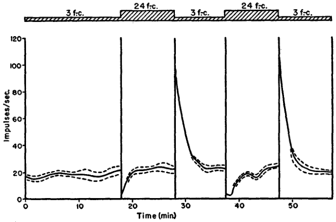
Figure 1: Figure 5 of Kuffler, Fitzhugh and Barlow (1957): Frequency of maintained discharge during changes of illumination. Off-center unit recorded with indium electrode. No permanent change of frequency resulted from change of illumination.

They then make a statistical description of the maintained discharge that looks like:

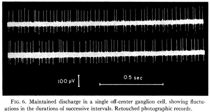
Figure 2: Figure 6 of Kuffler, Fitzhugh and Barlow (1957).

They propose a gamma distribution model for the inter spike intervals for the 'maintained discharge regime', we would say the stationary regime:

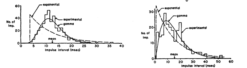
Figure 3: Figure 7 of Kuffler, Fitzhugh and Barlow (1957). Comparison of an 'nonparametric' probability density estimator (an histogram) with two theoretical models: an exponential plus a refractory or dead time and a gamma distribution. These are 2 cells among 6 that were analyzed in the same way.

Building a discharge model for the transient regime

In his 1958 paper, Fitzhugh wants first to build a discharge model for the transient parts of the neuron responses; that is, what is seen in the first above figure every time the light intensity is changed. Fitzhugh model boils down to:

The neuron has its own 'clock' whose rate is influenced by the stimulus that can increase it or decrease it (as long as the rate remains nonnegative).
The neuron always discharge following an renewal process with a fixed gamma distribution with respect to its own time (the time given by its clock).
Since the clock rate can be modified by a stimulus, the neuron time can be 'distorted'–the distortion is given by the integral of the rate–with respect to the 'experimental time' and the spike times generated by the neuron can be nonstationary and exhibit correlations.

Fitzhugh illustrates the working of his model by assuming the following rate (clock) function \(f\):

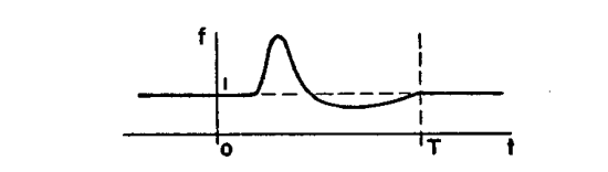
Figure 4: Figure 1a of Fitzhugh (1958).

The way to generate the observed spike train assuming this rate function is illustrated next:

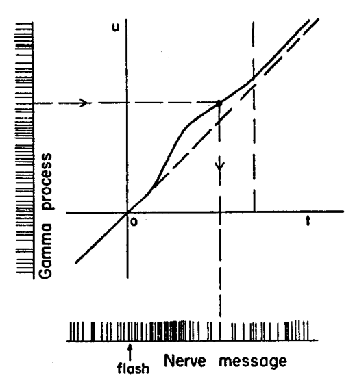
Figure 5: Figure 1b of Fitzhugh (1958).

You can see on the ordinate the realization of a renewal process with a gamma distribution. The curve that starts along the diagonal is the time distortion: \(u=f(t)\) is the neuron's time and \(f'\) is its clock rate. The observed process is obtained by mapping each spike time \(u_i\) of the gamma renewal process (ordinate) to the experimental time axis (abscissa) with \(t_i = f^{-1}(u_i)\) (since \(f'\) is nonnegative function, \(f\) is invertible).

Inference

Fitzhugh proposes to estimate \(f'\) from what we would now call a normalized version of the peri-stimulus time histogram. The normalization is done by setting the rate in the stationary regime to 1.

3.2. Your tasks

Towards of a replicate of Fitzhugh's figure (1)

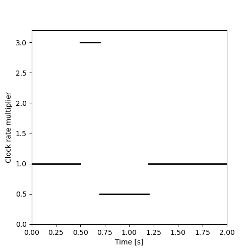
Use the following piecewise constant clock rate multiplier function (Fitzhugh's f(t)): \[[[0,1],[0.5,3],[0.7,0.5],[1.2,1]]\] where the Python list \([x,y]\) means that on the right (and including) \(x\) the rate value is \(y\). This piecewise constant is drawn on the next figure.

import matplotlib.pylab as plt
plt.figure(figsize=(5, 5))
plt.plot([0,0.5],[1,1],color='black',lw=2)
plt.plot([0.5,0.7],[3,3],color='black',lw=2)
plt.plot([0.7,1.2],[0.5,0.5],color='black',lw=2)
plt.plot([1.2,2.0],[1,1],color='black',lw=2)
plt.ylim([0,3.2])
plt.xlim([0,2.0])
plt.xlabel("Time [s]")
plt.ylabel("Clock rate multiplier")
plt.savefig("figs/ExFitzhughQ1a.png")
"figs/ExFitzhughQ1a.png"

Define first a piecewise linear function F(t) returning the integral of f(t) and test it. Next, define function inv_F(u) returning the inverse of F(t) and test it. Once you're happy with your functions, define a class PicewiseLinear with the following method:

__init__

(the constructor) takes two parameters:

a list of breakpoints (\([0,0.5,0.7,1.2]\) in our case),
a list of derivative values giving the value at and to the right of each breakpoint (\([1,3,0.5,1]\) in our case).

value_at

taking a single parameter, the time \(t\), and returning the value of the integral at that time–that is, the equivalent of function F(t) you practiced with–.

reciprocal_at

taking a single parameter, the 'neuron time' \(u\) and returning the inverse of the integral at \(u\) –that is, the equivalent of function inv_F(u) you practiced with–.

Check that your method implementation works.

Towards of a replicate of Fitzhugh's figure (2)

You are now ready to replicate Fitzhugh's figure. Take unit 3 of \citet[table 1, p. 696]{Kuffler_1957} whose discharge is well approximated by a renewal process with a gamma interval distribution: \[f(t) = \frac{k^a t^{a-1}}{\Gamma(a)} e^{-kt},\] with \(a = 8.08\) and \(k = 0.653\) [1/ms]. Then make a figure similar to figure 1 of \citet{Fitzhugh_1958} using the piecewise constant clock rate multiplier function considered at the beginning of this exercise and simulating an experimental time of 2 s.

Hints:

Function gammavariate of the random module of the standard library might be useful (check what the parameters of gammavariate mean!).
Don't forget to seed your (pseudo)random number generator.
The use of matplotlib eventplot function can save you a lot of time to make your raster plots.

Testing Fitzhugh's inference method

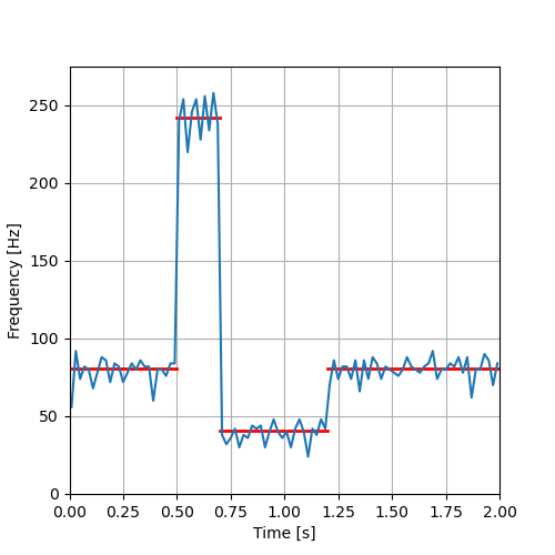
Fitzhugh's argues that if the same stimulation–that is, the same f(t) – is repeated \(n\) times, the peri-stimulus time histogram\index{peri-stimulus time histogram} (PSTH)\index{PSTH} is an estimator of a scaled version of the clock rate multiplier function f(t). The scaling factor being the rate of the underlying gamma process or the inverse of the mean interval of the gamma distribution (of the process). The PSTH is formally constructed as follows:

Assume that the stimulus is repeated \(R\) times in identical conditions and that data (spike times) are recorded between 0 and \(T\).
Each repetition gives rise to a spike train:
- Repetition 1: \(\{t_1^1,t_2^1,\ldots,t_{n_1}^1\}\)
- Repetition 2: \(\{t_1^2,t_2^2,\ldots,t_{n_2}^2\}\)
- …
- Repetition R: \(\{t_1^R,t_2^R,\ldots,t_{n_R}^R\}\)
- In general, \(n_1 \neq n_2 \neq \cdots \neq n_R\)
The \(n_{total} = n_1, n_2, \ldots, n_R\) spikes are put in the same set and ordered (independently of the repetition of origin) giving an aggregated train: \(\{t_1,t_2,\ldots,t_{n_{total}}\}\).
Interval \([0,T]\) is split (or partitioned) into \(K\) bins, typically, but not necessarily, of the same length, say \(\delta\).
The PSTH is then the sequence of bin counts (the number of spike times of the aggregated train falling in each bin) divided by \((R \times \delta)\).

Now that you know how to simulate one 'distorted gamma renewal process', you to not 1 but 25 simulations, build the corresponding PSTH using for instance a bin length (\(\delta\)) of 20 ms and compare it to Fitzhugh's claim.

Hint: the bin count required for building the interval is easily obtained once the (aggregated) counting process sample path (\(N(t)\)) has been constructed (as we did in exercise The inter mepp data of Fatt and Katz (1952); if \(t_l\) and \(t_r\) are the times of the left and right boundaries of a given bin, the bin count is just \(N(t_r)-N(t_l)\).

4. Solution 2: A Method Proposed by Fitzhugh in 1958

4.1. A remark

The coding style used in my solution is deliberately elementary and I avoid as much as I can the use of numpy and scipy. The concern here is twofold:

By coding things yourself instead of using blackbox functions, you are more likely to understand how things work.
Typically numpy codes break within 2 years while scipy ones can break after 6 months (because these huge libraries are evolving fast without a general concern for backward compatibility); by sticking to the standard library as much as I can, I hope that the following codes will run longer.

You are of course free to use more sophisticated libraries if you want to.

4.2. Towards of a replicate of Fitzhugh's figure (1)

Let's start by defining a piecewise linear function F(t) that returns the integral of Fitzhugh's clock rate multiplier function f(t). For now, we are going to do that in a 'messy' way letting our function depend on two variables defined in the global environment:

f_breakpoints: a list containing the breakpoints of f( ), [0,0.5,0.7,1.2],
f_values: a list with the same number of elements as f_breakpoints that contains the \linebreak f( ) values at the breakpoints and to the right of them, [1,3,0.5,1].

The reason why we allow ourselves this messy approach is that we will pretty soon define a class PiecewiseLinear and the instances of that class will contain theses two lists as 'private data'.

Remember that as soon as one deals with piecewise functions, using the functions defined in the bisect module of the standard library is a good idea. We start by assigning the two lists in our working environment:

f_breakpoints = [0,0.5,0.7,1.2]
f_values = [1,3,0.5,1]

We define our F function:

def F(t):
    import bisect
    if (t<f_breakpoints[0]) :
        return 0
    # We get the integral value at each
    # breakpoint
    F_values = [0]*len(f_breakpoints)
    F_values[0] = 0
    for i in range(1,len(f_breakpoints)):
        delta_t = f_breakpoints[i]-f_breakpoints[i-1]
        F_values[i] = F_values[i-1] + f_values[i-1]*delta_t
    # We get the index of the breakpoint <= t    
    left_idx = bisect.bisect(f_breakpoints,t)-1
    left_F = F_values[left_idx]
    delta_t = t-f_breakpoints[left_idx]
    return left_F + delta_t*f_values[left_idx]

We test it with:

[round(F(t),2) for t in [-1] + f_breakpoints + [2.0]]

[0, 0, 0.5, 1.1, 1.35, 2.15]

We define next the inverse of F, inv_F (note that the first part of the code is almost identical to the previous one):

def inv_F(u):
    import bisect
    # We get the integral value at each
    # breakpoint
    F_values = [0]*len(f_breakpoints)
    F_values[0] = 0
    for i in range(1,len(f_breakpoints)):
        delta_t = f_breakpoints[i]-f_breakpoints[i-1]
        F_values[i] = F_values[i-1] + f_values[i-1]*delta_t
    # We get the index of the breakpoint <= u    
    import bisect
    left_idx = bisect.bisect(F_values,u)-1
    left_t = f_breakpoints[left_idx]
    delta_u = u - F_values[left_idx]
    return left_t + delta_u/f_values[left_idx]

We test it by checking that inv_F(F(t)) is t:

[round(inv_F(F(t)),15) for t in f_breakpoints + [2.0]]

[0.0, 0.5, 0.7, 1.2, 2.0]

So to gain efficiency by avoiding recomputing F_values every time, let us define a PiecewiseLinear class with a value_at method (our previous F) and a reciprocal_at method (our previous inv_F):

class Piecewiselinear:
    """A class dealing with neurons clock rates"""
    <<init_method_pwl>>
    <<value_at-method-pwl>>
    <<reciprocal_at-method-pwl>>

`<<init_method_pwl>>`

The __init__ method is:

def __init__(self,breakpoints,values):
     import bisect
     n = len(breakpoints)
     if (n != len(values)):
         raise ValueError('breakpoints and values must have the same length.')

     Values = [0]*n
     Values[0] = 0

     for i in range(1,n):
         delta_t = breakpoints[i]-breakpoints[i-1]
         Values[i] = Values[i-1] + values[i-1]*delta_t

     self.breakpoints = breakpoints
     self.values = values
     self.Values = Values
     self.n = n

`<<value_at-method-pwl>>`

The value_at-method-pwl method:

def value_at(self,t):
    """Clock rate integral at t

    Parameters:
    -----------
    t: time

    Returns:
    --------
    Clock rate integral at t
    """
    import bisect
    left_idx = bisect.bisect(self.breakpoints,t)-1
    if (left_idx < 0): return 0
    left_F = self.Values[left_idx]
    delta_t = t-self.breakpoints[left_idx]
    return left_F + delta_t*self.values[left_idx]

`<<reciprocal_at-method-pwl>>`

The reciprocal_at-method-pwl method:

def reciprocal_at(self,u):
    """Reciprocal of clock rate integral at u

    Parameters:
    -----------
    u: 'neuron time'

    Returns:
    --------
    Reciprocal of clock rate integral at u
    """
    import bisect
    left_idx = bisect.bisect(self.Values,u)-1
    left_t = self.breakpoints[left_idx]
    delta_u = u - self.Values[left_idx]
    return left_t + delta_u/self.values[left_idx]

Some tests

We check it by repeating the previous tests:

pwl = Piecewiselinear(f_breakpoints,f_values)
[round(pwl.value_at(t),2) for t in [-1] + f_breakpoints + [2.0]]

[0, 0, 0.5, 1.1, 1.35, 2.15]

[round(pwl.reciprocal_at(pwl.value_at(t)),15) for t in f_breakpoints + [2.0]]

[0.0, 0.5, 0.7, 1.2, 2.0]

4.3. Towards of a replicate of Fitzhugh's figure (2)

We need first to know for how long we must simulate on the 'neuronal time' and this time is given by the integral of the clock rate, namely:

pwl.value_at(2.0)

2.15

We now simulate a gamma renewal process for a duration of 2.15 s. To that end, we use function gammavariate of the random module of the standard library. We do not forget to set the seed of our (pseudo-)random number generator; we are also carrefull with the different parametrisation used by gammavariate whose beta parameter is the inverse of the parameter k of the gamma distribution density given in the exercise statement. Finally, the latter statement gives k in 1/msec while the time unit of the exercise is the second. With that in mind we do:

import random
random.seed(20110928)  # set the seed
train = []
current_time = 0
beta = 1/0.653/1000 # take care of parametrization and time unit
while current_time < 2.15:
    current_time += random.gammavariate(8.08,beta)
    train += [current_time]

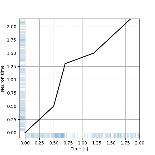
We then need to mapp this renewal process in 'neuron time' into the experimental time. To that end, we use our reciprocal_at method and we want to have the mapped sequence: \(\{t_1=f^{-1}(u_1),t_2=f^{-1}(u_2),\ldots,t_n=f^{-1}(u_n)\}\). We can then get the spike times on the 'experimental time scale':

mapped_train = [pwl.reciprocal_at(u) for u in train]

To make a figure similar to Fitzhugh's one, we use matplotlib eventplot function as follows:

plt.figure(figsize=(5, 5))
plt.plot([0,0.5],[pwl.value_at(0),pwl.value_at(0.5)],color='black',lw=2)
plt.plot([0.5,0.7],[pwl.value_at(0.5),pwl.value_at(1.1)],color='black',lw=2)
plt.plot([0.7,1.2],[pwl.value_at(1.1),pwl.value_at(1.35)],color='black',lw=2)
plt.plot([1.2,2.0],[pwl.value_at(1.35),pwl.value_at(2.15)],color='black',lw=2)
plt.eventplot(mapped_train,orientation='horizontal',
              lineoffsets=-0.05,linelengths=0.1,linewidths=0.3)
plt.eventplot(train,orientation='vertical',
              lineoffsets=-0.05,linelengths=0.1,linewidths=0.3)
plt.grid()
plt.ylim([-0.1,2.15])
plt.xlim([-0.1,2.0])
plt.xlabel("Time [s]")
plt.ylabel("Neuron time")
plt.savefig('figs/ExFitzhughQ1a_solution.png')
'figs/ExFitzhughQ1a_solution.png'

4.4. Testing Fitzhugh's inference method

We start with the simulations. To that end we create a function that generates a 'mapped gamma renewal process', that is, that generates first a gamma renewal process (on the 'neuron time') before mapping that process on the 'experimental time':

def mapped_gamma_renewal_process(alpha,beta,total_time,pwl):
    """Generate a mapped gamma renewal process

    Parameters:
    -----------
    alpha: the shape parameter of the distribution
    beta: the scale parameter of the distribution
    total_time: the duration to simulate
    pwl: a PiecewiseLinear class instance

    Results:
    --------
    A list of event times
    """
    import random
    # We get the simulation duration
    duration = pwl.value_at(total_time)
    # We generate first a gamma distributed renewal process
    # on the 'neuron time scale'
    train = []
    current_time = 0
    while current_time < duration:
        current_time += random.gammavariate(alpha,beta)
        train += [current_time]
    return [pwl.reciprocal_at(u) for u in train]

We test it by regenerating our former simulation:

random.seed(20110928)  # set the seed at the same value as before
alpha = 8.08
mapped_train2 = mapped_gamma_renewal_process(alpha,beta,2.0,pwl)
all([mapped_train[i] == mapped_train2[i] for i in range(len(mapped_train))])

True

Fine, so we make the 25 replicates:

random.seed(20110928)
n_rep = 25
many_trains = [mapped_gamma_renewal_process(alpha,beta,2.0,pwl) for i in range(n_rep)]
sum([len(train) for train in many_trains])

We aggregate the 25 replicates and sort the result:

aggregated_train = many_trains[0]
for i in range(1,len(many_trains)): 
    aggregated_train.extend(many_trains[i])
aggregated_train.sort()
len(aggregated_train)

We then define class CountingProcess as in Answer Question 4: Counting Process Class and we create the requested instance:

class CountingProcess:
     """A class dealing with counting process sample paths"""
     def __init__(self,times):
          from collections.abc import Iterable
          if not isinstance(times,Iterable): # Check that 'times' is iterable
               raise TypeError('times must be an iterable.')
          
          n = len(times)
          diff = [times[i+1]-times[i] for i in range(n-1)]
          all_positive = sum([x > 0 for x in diff]) == n-1
          if not all_positive:  # Check that 'times' elements are increasing
               raise ValueError('times must be increasing.')
          
          self.cp = times
          self.n = n 
          self.min = times[0]
          self.max = times[n-1]
     
     def sample_path(self,t):
          """Returns the number of observations up to time t"""
          from bisect import bisect
          return bisect(self.cp,t)
     
     def plot(self, domain = None, color='black', lw=1, fast=False):
         """Plots the sample path
     
         Parameters:
         -----------
         domain: the x axis domain to show
         color: the color to use
         lw: the line width
         fast: if true the inexact but fast 'step' method is used
         
         Results:
         --------
         Nothing is returned the method is used for its side effect
         """
         import matplotlib.pylab as plt
         import math
         n = self.n
         cp = self.cp
         val = range(1,n+1)
         if domain is None:
             domain = [math.floor(cp[0]),math.ceil(cp[n-1])]
         if fast:
             plt.step(cp,val,where='post',color=color,lw=lw)
             plt.vlines(cp[0],0,val[0],colors=color,lw=lw)
         else:
             plt.hlines(val[:-1],cp[:-1],cp[1:],color=color,lw=lw)
         plt.xlim(domain)
         if (domain[0] < cp[0]):
             plt.hlines(0,domain[0],cp[0],colors=color,lw=lw)
         if (domain[1] > cp[n-1]):
             plt.hlines(val[n-1],cp[n-1],domain[1],colors=color,lw=lw)

ag_cp = CountingProcess(aggregated_train)

We create the PSTH using a 20 ms bin length:

delta = 0.02
norm_factor = 1/delta/n_rep
tt = [i*delta for i in range(101)]
histo_ag_cp = [(ag_cp.sample_path(tt[i+1])-
                ag_cp.sample_path(tt[i]))*norm_factor for i in range(100)]

We then plot the PSTH together with Fitzhugh's prediction:

plt.figure(figsize=(5, 5))
bt = [t+0.5*delta for t in tt[:-1]]
basal_rate= 1/alpha/beta
plt.plot([0,0.5],[basal_rate,basal_rate],color='red',lw=2)
plt.plot([0.5,0.7],[3*basal_rate,3*basal_rate],color='red',lw=2)
plt.plot([0.7,1.2],[0.5*basal_rate,0.5*basal_rate],color='red',lw=2)
plt.plot([1.2,2.0],[basal_rate,basal_rate],color='red',lw=2)
plt.plot(bt,histo_ag_cp)
plt.grid()
plt.xlim([0,2])
plt.ylim([0,275])
plt.xlabel("Time [s]")
plt.ylabel("Frequency [Hz]")
plt.savefig('figs/ExFitzhughQ4_solution.png')
'figs/ExFitzhughQ4_solution.png'